To understand these relationships, we need a way to quantify how sensitive one quantity is to changes in another: if we change one variable by a small amount, how much does another variable change in response?
Imagine you’re adjusting the volume knob in two different cars: your own car and your friend’s car. Let \(V\) be the volume of the music in decibels (dB), and let \(x\) be the number of millimeters you turn the knob to the right from the minimum-volume position. (More precisely, it’s how many millimeters you turn the outer edge of the knob.)
Suppose that in both cars, the volume ranges from \(0\) dB at the minimum setting up to \(80\) dB at the maximum setting. In your car, turning the knob \(40\) mm to the right brings the volume from \(0\) dB to \(80\) dB. In your friend’s car, however, you only have to turn the knob \(20\) mm to go from \(0\) dB to \(80\) dB. Hence the volume knob in your friend’s car is more sensitive.
We can quantify the sensitivity by calculating how many decibels the volume increases per millimeter of turning the knob. In your car, the volume increases from \(0\) dB to \(80\) dB when you turn the knob by \(40\) mm, so the sensitivity is
\begin{equation*}
\frac{80\text{ dB}}{40\text{ mm}}=2\text{ dB per mm}\text{.}
\end{equation*}
Meanwhile, in your friend’s car, the volume increases from \(0\) dB to \(80\) dB when you turn the knob by \(20\) mm, so the sensitivity is
\begin{equation*}
\frac{80\text{ dB}}{20\text{ mm}}=4\text{ dB per mm}\text{.}
\end{equation*}
Hence the volume in your friend’s car is more sensitive to changes in the knob position.
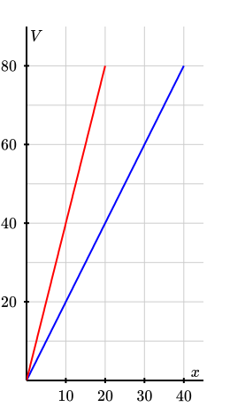
We can also visualize the sensitivity by looking at a graph. Suppose the blue line represents the volume in your car, while the red line represents the volume in your friend’s car.
The equation of the line for your car is \(V=2x\text{,}\) and the equation for your friend’s car is \(V=4x\text{.}\) Notice that the sensitivity is the slope of each line:
In the example above, the volume of the sound system was a linear function of the position of each knob, which means that the sensitivity was the same no matter which two points we chose to calculate it between. But what if we analyze a situation where the relationship is nonlinear?
Imagine you’re selling tickets for a small concert you’re organizing at your university. You’re currently charging \(\$3.00\) per ticket, but you wonder whether you should increase the price. You wonder, how sensitive would your revenue be to a change in the price?
Based on some market research, you find that the revenue \(R\) that you earn (in thousands of dollars) can be modeled by the function
\begin{equation*}
R = 4p - 0.25p^2\text{,}
\end{equation*}
where \(p\) is the price (in dollars) that you charge for each ticket. To emphasize that the revenue is a function of the price, we can also write this as
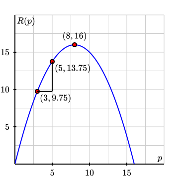
As the price begins to increase, your revenue increases as well, reaching a maximum of \(R=16\) (that is, \(\$16,\!000\)) when you charge \(\$8.00\) per ticket.
After the price exceeds \(\$8.00\text{,}\) the revenue starts to decrease, until at a price of \(\$16.00\text{,}\) consumers are no longer willing to buy tickets, and once again you earn no revenue.
Now, suppose you’re currently charging \(\$3.00\text{,}\) and you decide to raise the price to \(\$5.00\text{;}\) that is, the change in price (\(\Delta p\)) is
That is, the sensitivity is the ratio of the change in the output to the change in the input over that interval. We often say this out loud as ‘the sensitivity of \(y\) to the change in \(x\text{.}\)’
How do these sensitivites compare to the sensitivity we calculated above when the ticket price changes from \(\$3\) to \(\$5\text{?}\) What do you notice about the relationship between the sensitivity and the shape of the graph?
Our calculation of the sensitivity above was somewhat coarse: since the graph of \(R(p)\) is curved, the slope gets gradually steeper as we go along the curve. In other words, our calculation seems to mix together several sensitivities.
If we want a more fine-grained measurement, a natural idea is to look at smaller changes in price. Here’s what happens if we use a change in price of \(\Delta p=0.1\) dollars:
Estimate the sensitivity of the revenue to the following changes \(\Delta p\) (assuming an initial price of \(p\tsub{init}=3\) dollars). What do you notice about the values you get?
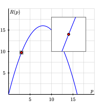
Over smaller and smaller changes, the graph looks more and more like a straight line, and the slope between the two points appears to approach a particular value, which seems to be around \(2.5\) thousand dollars earned per dollar charged. (We’ll soon learn how to find this value exactly, without having to do so many calculations.)
If we could do this, we might imagine that the graph of \(R(p)\) would be indistinguishable from a perfectly straight line at that point. So if we could somehow choose two points that are ‘infinitely close’ to each other, then the ratio of the infinitesimal (infinitely small) changes would be the slope of that line:
We call these infinitely small changes differentials, and we represent them with a lowercase \(\mathrm{d}\text{:}\) in this case, we would write \(\dd{p}\) to denote an infinitesimal change in price, and \(\dd{R}\) to denote the corresponding infinitesimal change in revenue. The ratio of these differentials would then be written
where \(b\) is ‘infinitely close’ to \(a\text{.}\) This definition is currently somewhat vague, as we have not defined what it means to be ‘infinitely close.’ We’ll make this definition more precise later.
When we want to emphasize that the sensitivity is being evaluated at a particular point \(x=a\text{,}\) we will write \(\eval{\DS\dv{y}{x}}_{x=a}\) or \(\eval{\DS\dv{f}{x}}_{x=a}\text{.}\)
Now, you might be a bit skeptical of this idea of using ‘infinitely small’ changes. If so, you’re in good company! This idea of using infinitesimal quantities has long been a controversial topic in mathematics. On one hand, infinity is notoriously difficult to get a handle on — just how small is ‘infinitely small’ anyway? On the other hand, allowing ourselves to work with these infinitesimal ideas has helped us solve a lot of tricky problems throughout history. By developing calculus, we’ll be able to find a way to make these intuitive-but-somewhat-vague arguments more precise; this will enable us to confidently use them to describe real-world phenomena in a variety of applied contexts.
Use this same process to estimate \(\eval{\DS\dv{R}{p}}_{p=5}\) and \(\eval{\DS\dv{R}{p}}_{p=9}\text{.}\) How does the sensitivity of revenue to changes in price compare at these different prices?
On the left side of the graph (when \(p \lt 8\)), the sensitivity \(\DS\dv{R}{p}\) is positive. This means that increasing the price would lead to an increase in revenue, and decreasing the price would lead to a decrease in revenue.
On the right side of the graph (when \(p \gt 8\)), the sensitivity \(\DS\dv{R}{p}\) is negative. This means that increasing the price would lead to a decrease in revenue, and decreasing the price would lead to an increase in revenue.
We can also use the sensitivity to estimate how much the revenue will change to a small change in price. For example, suppose that at a price of \(\$9.00\text{,}\) we know that the sensitivity is
\begin{equation*}
\eval{\DS\dv{R}{p}}_{p=9} = -0.5\text{ thousand dollars earned per dollar charged}\text{.}
\end{equation*}
Now suppose we want to raise the price from \(\$9.00\) to \(\$9.10\text{.}\) Since the sensitivity \(\DS\dv{R}{p}\) is supposed to be the ratio of ‘infinitely small’ changes, we can write:
Hence if we increase the price from \(\$9.00\) to \(\$9.10\text{,}\) we can estimate that the revenue will decrease by approximately \(\$50.00\text{.}\)
So our estimate of a \(\$50.00\) decrease in revenue was pretty close to the actual decrease of about \(\$52.50\text{.}\) However, computing the actual decrease required we compute the revenue at two different prices, and for a different change in price, we’d need to compute a new revenue every single time. On the other hand, using the sensitivity at a point lets us make lots of quick estimates of how the revenue will change in response to small changes in price without having to recompute the revenue every time.
Suppose that we decide to decrease the price from \(\$9.00\) to \(\$8.95\text{.}\) How much would we estimate the revenue to change? Would it increase or decrease? Use the sensitivity at \(p=9\) to justify your answer.
In this exercise, you’ll interpret the sign of the sensitivity for various real-world contexts. For each one, determine whether the sensitivity should be positive, negative, or zero, and explain your answer. (Think: if you increase the independent variable, what would you expect to happen to the dependent variable?) Also give the units for the sensitivity.
\(\DS\dv{B}{P}\text{,}\) where \(B=\) the brightness of a lamp (measured in lumens) and \(P=\) the electrical power supplied to the lamp (measured in watts)
\(\DS\dv{T}{t}\text{,}\) where \(T=\) the temperature (in degrees Fahrenheit) of a baked potato and \(t=\) the number of minutes for which the potato is left to bake in the oven
\(\DS\dv{t}{T}\text{,}\) where \(t=\) the number of minutes it takes to fully bake a potato (i.e. to get it to reach a desired temperature) and \(T=\) the temperature (in degrees Fahrenheit) of the oven
It can be shown that in the ticket example, the quantity demanded of tickets (the number of tickets that consumers are willing to buy, measured in thousands of tickets) is a function of the price, given by \(x(p)=4-0.25p\text{.}\) The revenue is then given by
Suppose \(y=5\text{,}\) so \(y\) is a constant function of \(x\text{.}\) That is, no matter what the value of \(x\) is, the value of \(y\) is always \(5\text{.}\)
If \(y=k\) is a constant function of \(x\text{,}\) where \(k\) is any constant, what will the sensitivity of \(y\) be at any point \(x=a\text{?}\) Why?
Estimate \(\DS\dv{y}{x}\) at the point \(x=1\) by computing the ratios of small changes in the input and output. As the intervals get smaller and smaller, what number does the sensitivity seem to be approaching?
Repeat the above exercise to estimate \(\DS\dv{y}{x}\) at the points \(x=2\) and \(x=3\text{.}\) What do you notice about the values you get for the sensitivity at these different points?
Estimate \(\DS\dv{y}{x}\) for each of the following graphs at the given points by computing the ratios of small changes in the input and output. As the intervals get smaller and smaller, what number do the sensitivities seem to be approaching?
Suppose the temperature in the Pacific Ocean can be described by the function \(T(\ell)\text{,}\) where \(T\) is the temperature in degrees Celsius and \(\ell\) is the latitude in degrees.
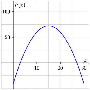
The profit earned by a company can be defined as the revenue (the money it brings in) minus the costs (the money it spends). The graph below shows \(P(x)\text{,}\) the profit (in thousands of dollars) earned by a company as a function of \(x\text{,}\) the number of units produced (in hundreds of units).
For which values of \(x\) does \(P(x)\) appear to be positive? What about negative? Explain how you can tell from the graph. What do these values mean practically for the company?
For which values of \(x\) does \(\DS\dv{P}{x}\) appear to be positive? What about negative? Explain how you can tell from the graph. What do these values mean practically for the company?
Based on the graph, about how many units should the company produce in order to maximize profit, and what is that maximum profit? What is \(\DS\dv{P}{x}\) at that point?
A car is driven along a fixed 100-mile route. The table below shows the total amount of energy \(E\) used for the trip as a function of the car’s speed \(v\text{.}\) Here \(v\) is measured in miles per hour and \(E\) is measured in kilowatt-hours.
Suppose we know that the energy usage is minimized when \(v=55\) mph. What would you expect the value of \(\DS\dv{E}{v}\) to be at that speed? Explain.