Skip to main content
Contents Embed Dark Mode Prev Up Next \(\require{physics}\require{upgreek}\everymath{\displaystyle}
\newcommand{\N}{\mathbb N}
\newcommand{\Z}{\mathbb Z}
\newcommand{\Q}{\mathbb Q}
\newcommand{\R}{\mathbb R}
\newcommand{\inv}{^{-1}}
\newcommand{\DS}{\displaystyle}
\newcommand{\eps}{\varepsilon}
\newcommand{\tsub}[1]{_{\mathrm{#1}}}
\newcommand{\ee}{\mathrm{e}}
\newcommand{\ii}{\mathrm{i}}
\newcommand{\limit}[1]{\lim\limits_{#1}}
\newcommand{\resid}[1]{\underset{#1}{\Res}}
\DeclareMathOperator{\sinc}{sinc}
\DeclareMathOperator{\sgn}{sgn}
\newcommand{\pii}{\pi}
\DeclareMathOperator{\Prob}{P}
\DeclareMathOperator{\EV}{E}
\DeclareMathOperator{\Var}{Var}
\newcommand{\bv}[1]{\boldsymbol{#1}}
\newcommand{\uv}[1]{\hat{\bv{#1}}}
\newcommand{\cl}[1]{\mathcal{#1}}
\newcommand{\bb}[1]{\mathbb{#1}}
\DeclareMathOperator{\Cis}{cis}
\DeclareMathOperator{\RE}{Re}
\DeclareMathOperator{\IM}{Im}
\newcommand{\xd}{\mathbf{d}}
\newcommand{\seq}[3]{{#1}_{#2},\cdots,{#1}_{#3}}
\newcommand{\psup}[1]{^{(#1)}}
\newcommand{\hypext}{{}^*}
\DeclareMathOperator{\st}{st}
\newcommand{\set}[1]{\left\{#1\right\}}
\DeclareMathOperator{\Sin}{Sin}
\DeclareMathOperator{\Cos}{Cos}
\DeclareMathOperator{\Tan}{Tan}
\DeclareMathOperator{\Sec}{Sec}
\DeclareMathOperator{\Csc}{Csc}
\DeclareMathOperator{\Cot}{Cot}
\DeclareMathOperator{\Log}{Log}
\DeclareMathOperator{\Arg}{Arg}
\DeclareMathOperator{\Ln}{Ln}
\DeclareMathOperator{\Grad}{grad}
\DeclareMathOperator{\Div}{div}
\DeclareMathOperator{\Curl}{curl}
\newcommand{\rd}{\textstyle\mathop{}\!\mathrm{d}^{\!\!\!-}\hspace{-0.0555 em}}
\newcommand{\rpd}{\textstyle\mathop{}\!\partial^{\hspace{-0.5 em}-}\hspace{-0.1666 em}}
\newcommand{\rdv}[2]{\frac{\rd{#1}}{\rd{#2}}}
\newcommand{\rpdv}[2]{\frac{\rpd{#1}}{\rpd{#2}}}
\newcommand{\lt}{<}
\newcommand{\gt}{>}
\newcommand{\amp}{&}
\definecolor{fillinmathshade}{gray}{0.9}
\newcommand{\fillinmath}[1]{\mathchoice{\colorbox{fillinmathshade}{$\displaystyle \phantom{\,#1\,}$}}{\colorbox{fillinmathshade}{$\textstyle \phantom{\,#1\,}$}}{\colorbox{fillinmathshade}{$\scriptstyle \phantom{\,#1\,}$}}{\colorbox{fillinmathshade}{$\scriptscriptstyle\phantom{\,#1\,}$}}}
\)
Section 16.3 Visualizing complex functions
Objectives
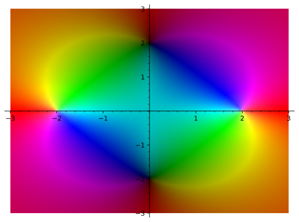
Visualize complex mappings using domain coloring to encode magnitude and argument.
Extend the complex plane to the Riemann sphere by adding a point at infinity.
Break down complex functions into their real and imaginary parts.
Domain coloring: Let the input be the point on the complex plane, and let the output be how we color it.
Lightness = modulus (black =
\(0\text{,}\) full color =
\(1\text{,}\) white =
\(\infty\) )
Hue = argument (red =
\(0\text{,}\) lime =
\(\pii/2\text{,}\) cyan =
\(\pii\text{,}\) purple =
\(3\pii/2\)
Powers using De Moivre’s formula:
\begin{equation*}
(r\ee^{\ii\theta})^{n}=r^{n}\ee^{n\ii\theta}
\end{equation*}
Roots of unity:
\(z^n=1\) has roots at
\(\ee^{2\pii\ii k/n}\) for
\(k=0,1,\ldots,n-1\text{.}\)
We can see this in the domain coloring of
\(z^n-1\text{,}\) where the colors cycle around the unit circle and approach black (zero) at the roots of unity.
Focus on \(f(z)=\dfrac{1}{z}\text{.}\)
Domain coloring: Swaps light and dark, and colors cycle the other way.
Division by zero and the Riemann sphere
Define a pole of a function as a zero of its reciprocal. But need to find a slightly different way to say this, as it’s missing some things.
Look at domain coloring plots of other complex functions, focusing on zeros and poles, perhaps as well as other stranger singularities (such as
\(\ee^{-1/z}\) ).