In the ancient world, mathematicians needed the answer to this question to design things like temples, storage containers, and astronomical instruments. They of course knew how to calculate areas of simple shapes like rectangles and triangles, as well as polygons that could be broken into these shapes. But a circle has no straight sides, so it doesn’t naturally decompose into those familiar pieces.
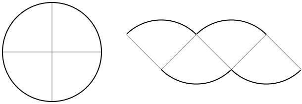
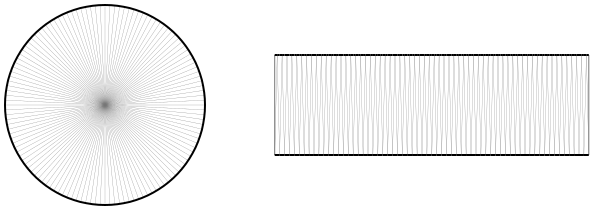
A natural idea might be to see what pieces you can break a circle into. You might start by slicing it into four equal wedges, as in the figure below. If we rearrange those pieces, alternating between pointing them up and down, we get a shape that resembles a parallelogram.
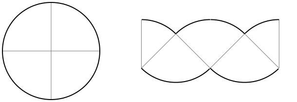
If we then slice one of those pieces down the middle and move it to the other side, we have a shape with two vertical sides and a bumpy top and bottom.
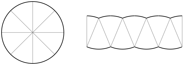
What if we slice the circle into eight wedges instead of four? If we follow the same process as earlier, the shape we get has smaller, more gentle bumps along the top and the bottom:
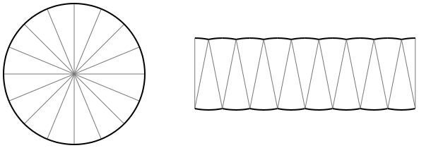
Each time we increase the number of wedges, the rearranged figure starts to look more and more like a rectangle, with the curved boundary of the original circle being distributed across many tiny pieces.
In that case, you might imagine that the top and bottom wouldn’t look bumpy at all. You wouldn’t be able to tell the difference between the rearranged figure and a rectangle, no matter how closely you zoomed in. And since area doesn’t change when we just rearrange the pieces, the area of this rectangle should be the same as the area of the original circle.
We can identify that the height of the rectangle is the radius \(r\) of the circle, and the base is half the circumference \(C\) of the circle, since the circle’s boundary has been distributed across the top and bottom of the rectangle. So the rectangle has area
Notice that we’ve reduced the problem of finding the area of a circle to the problem of finding its circumference. And since the circumference of a circle is proportional to its radius, once we know that constant of proportionality, we can determine the area of a circle from its radius alone. In the exercises below, you’ll see how to find this constant by approximating the boundary of the circle with polygons.
If you had any of these concerns, you’re in good company! This idea of using infinitesimal (infinitely small) pieces has long been a controversial topic in mathematics. On one hand, infinity is notoriously difficult to get a handle on; on the other hand, allowing ourselves to work with these infinitesimal ideas has helped us solve a lot of tricky problems throughout history. Out of centuries of wrestling with these ideas came the field that today we call calculus, and that is what we’ll be studying throughout this book. By developing calculus, we’ll be able to find a way to make these intuitive-but-somewhat-vague arguments more precise, which will allow us to use them with confidence to solve problems in a variety of applied contexts.
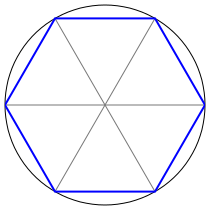
In this exercise, we will approximate the circumference of a unit circle by inscribing polygons with an increasing number of sides. This method is due to Liu Hui, a Chinese mathematician who lived in the third century AD. It doesn’t require any trigonometry — just the Pythagorean theorem and some algebra.
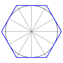
Remember that a regular hexagon has six equal sides and six equal angles. If you split it into six triangles as shown, what kind of triangle do you get?
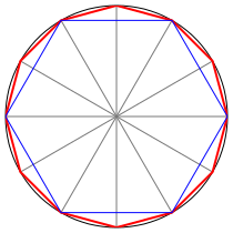
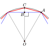
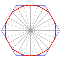
Continue this process of bisecting arcs to get a regular \(24\)-sided polygon, then a regular \(48\)-sided polygon, and finally a \(96\)-sided polygon. What do you notice about the perimeters of these polygons?
(Hint: You probably won’t be able to actually draw these polygons. Instead, use the lengths from each step to find the lengths needed for the next step.)
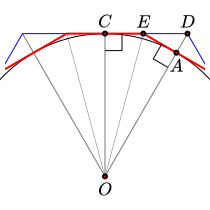
We can also approximate the circumference of a unit circle by circumscribing polygons with an increasing number of sides. These sides are tangent to the circle, meaning they barely touch the circle at a single point. Notice that each tangent line makes a right angle with the radius of the circle where it touches.
Suppose we bisect each of the six arcs of the circle and construct a tangent line to the circle at each of these points, giving a regular dodecagon circumscribed around the circle, as shown below.
Continue this process of bisecting arcs and constructing tangent lines to get a regular \(24\)-sided polygon, then a regular \(48\)-sided polygon, and finally a \(96\)-sided polygon. What do you notice about the perimeters of these polygons?
How does this method of approximating the circumference compare to the method of inscribed polygons? Do you think they’re guaranteed to give the same result? Why or why not?
Repeat the above exercises, but this time start with an inscribed square and a circumscribed square instead of a hexagon. How do the results compare to the previous exercises?
Remember that the equation of a circle of radius \(1\) in the plane is given by \(x^2 + y^2 = 1\text{,}\) so the upper semicircle has equation \(y = \sqrt{1 - x^2}\text{.}\)
How does this method compare to the method of inscribed or circumscribed polygons? Do you think they’re guaranteed to give the same result? Why or why not?
The process in the first exercise can be expressed using a recurrence relation as follows: If the perimeter of the inscribed polygon with \(n\) sides is \(P_n\text{,}\) then the perimeter of the inscribed polygon with \(2n\) sides is given by
Write a computer program to implement these recurrence relations and use it to compute perimeters of inscribed and circumscribed polygons with more and more sides. How do these values compare to \(\tau\) as you increase the number of sides?